The multinomial probit (MNP) replaces logit’s Type-I extreme-value error structure with a multivariate-normal covariance for utility differences. That covariance can encode correlated substitution across alternatives. The cost is scale normalization, a covariance parameterization that grows quickly with the number of alternatives, and MCMC diagnostics. choicer estimates the model the Bayesian way: a Gibbs sampler with data augmentation, written in C++ with a reproducible, thread-safe random number generator.
Simulate from a probit process
simulate_mnp_data() draws choices with correlated normal
errors and known parameters.
sim <- simulate_mnp_data(N = 2000, J = 3, seed = 1)
sim
#> <choicer_sim: mnp>
#>   settings:
#>     N = 2000
#>     J = 3
#>     K_x = 2
#>     base_alt = 1
#>   rows in $data: 6000
#>   true_params: beta, delta, Sigma
Run the sampler
run_mnprobit() returns posterior draws. The settings
below keep this vignette quick; for real work use a longer run, repeat
the fit with several independent seeds when needed, and inspect trace,
autocorrelation, ESS and Monte Carlo error before interpreting posterior
summaries. run_mnprobit() does not currently expose
user-specified starts or a multi-chain wrapper.
set.seed(3)
fit <- run_mnprobit(
  data           = sim$data,
  id_col         = "id",
  alt_col        = "alt",
  choice_col     = "choice",
  covariate_cols = c("x1", "x2"),
  mcmc           = list(R = 4000, burn = 1000, thin = 2)
)
#> MCMC run time 0h:0m:0.54s
summary(fit)
#> Bayesian Multinomial Probit (MNP) model
#>
#> Parameter        Mean         SD       2.5%     Median      97.5%
#> x1           0.783220   0.045629   0.695931   0.782835   0.874073
#> x2          -0.583254   0.040918  -0.662456  -0.581719  -0.506304
#> ASC_2        0.473710   0.043612   0.384752   0.474199   0.558204
#> ASC_3       -0.534590   0.105388  -0.783720  -0.521079  -0.361807
#>
#> Covariance of utility differences (Sigma, identified scale):
#> Parameter        Mean         SD       2.5%     Median      97.5%
#> Sigma_11     1.000000   0.000000   1.000000   1.000000   1.000000
#> Sigma_21     0.416625   0.134911   0.112042   0.428090   0.670017
#> Sigma_22     1.410789   0.273690   0.957033   1.385073   1.988667
#>
#> Posterior mean Sigma:
#>        w_2    w_3
#> w_2 1.0000 0.4166
#> w_3 0.4166 1.4108
#>
#> Base alternative: 1
#> Draws kept: 1500 (R = 4000, burn = 1000, thin = 2, seed = 721735354)
#> N: 2000  | Parameters: 4
#> Sampling time: 0.54 s
#> Identification: per-draw normalization by sigma_11 (McCulloch-Rossi 1994).
The Sigma entries are the error-covariance parameters.
They are identified only up to scale, so choicer reports them on the
normalized scale where Sigma_11 = 1. The prior is placed on
the unrestricted covariance used inside the Gibbs sampler; the reported
posterior summaries are computed after normalizing each kept draw.
For empirical work, ask what disciplines the covariance before interpreting it. Keane (1992) shows that when covariates do not vary across alternatives — demographics, or constants alone — the covariance parameters are identified by the normal functional form only, and estimation is fragile. Alternative-specific covariate variation (prices, distances, or attributes that differ across the options within a choice situation), and especially defensible exclusions across utility equations, is what separates covariance from systematic utility in practice; the simulated data above contain two varying attributes. The Bayesian machinery does not repeal this: with weak alternative-specific variation the posterior sits close to its prior, and the substitution pattern it implies is maintained rather than estimated. The MNP is attractive when flexible error correlation is the central object, but with many alternatives its parameter count rises quickly.
Compare posterior summaries with the truth
recovery_table(fit, sim$true_params)
#> <choicer_recovery> model=choicer_mnp level=0.95
#>    parameter  group  true estimate     se    bias rel_bias_pct z_vs_true
#>       <char> <char> <num>    <num>  <num>   <num>        <num>     <num>
#> 1:        x1   beta   0.8   0.7832 0.0456 -0.0168       -2.097   -0.3677
#> 2:        x2   beta  -0.6  -0.5833 0.0409  0.0167       -2.791    0.4093
#> 3:     ASC_2    asc   0.5   0.4737 0.0436 -0.0263       -5.258   -0.6028
#> 4:     ASC_3    asc  -0.5  -0.5346 0.1054 -0.0346        6.918   -0.3282
#> 5:  Sigma_11  sigma   1.0   1.0000 0.0000  0.0000        0.000        NA
#> 6:  Sigma_21  sigma   0.5   0.4166 0.1349 -0.0834      -16.675   -0.6180
#> 7:  Sigma_22  sigma   1.5   1.4108 0.2737 -0.0892       -5.947   -0.3260
#>    lower_ci upper_ci covers
#>       <num>    <num> <lgcl>
#> 1:   0.6938   0.8727   TRUE
#> 2:  -0.6635  -0.5031   TRUE
#> 3:   0.3882   0.5592   TRUE
#> 4:  -0.7411  -0.3280   TRUE
#> 5:   1.0000   1.0000   TRUE
#> 6:   0.1522   0.6810   TRUE
#> 7:   0.8744   1.9472   TRUE
In this simulated example the posterior summaries line up with the parameters that generated the data. As with the frequentist recovery vignettes, this is an illustration rather than a proof: what matters in repeated use is posterior coverage, mixing, and sensitivity to prior and normalization choices.
A quick MCMC diagnostic
Posterior draws are stored on the fit, so the usual diagnostics are a line away. A trace plot of the price coefficient should look like a stationary “fuzzy caterpillar”:
beta_draws <- fit$draws$beta
plot(beta_draws[, "x2"], type = "l", col = "steelblue",
     xlab = "iteration", ylab = expression(beta[x2]),
     main = "Posterior trace: price coefficient")
abline(h = sim$true_params$beta[2], col = "red", lwd = 2)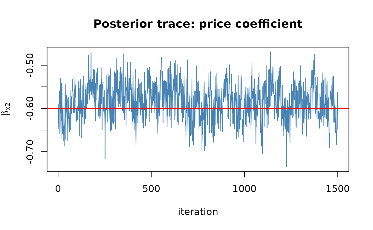
The red line marks the true value; the chain should hover around it.
The same diagnostics used for the hierarchical models apply to any draws
matrix: rhat() computes the split R-hat (values near 1 are
consistent with convergence) and ess() the rank-normalized
bulk and tail effective sample sizes — the number of effectively
independent draws behind each posterior summary:
rhat(fit$draws$beta)
#>     x1     x2  ASC_2  ASC_3
#> 1.0017 1.0171 0.9998 1.0190
ess(fit$draws$beta)
#>         bulk  tail
#> x1    164.40 578.6
#> x2    137.55 420.9
#> ASC_2  86.50 169.6
#> ASC_3  55.58  68.1
mcse(fit$draws$beta)
#>       x1       x2    ASC_2    ASC_3
#> 0.003559 0.003489 0.004689 0.014136
On a single chain these are necessary rather than sufficient checks;
the stronger practical check in the current API is to repeat the
complete fit with several independent seeds, then compare posterior
summaries and pass equal-length draw matrices as a list to the same
diagnostic functions, for example
rhat(list(fit$draws$beta, fit_seed_2$draws$beta), rank = TRUE).
Because the sampler’s initial state is internal rather than
user-controlled, this is not equivalent to deliberately overdispersed
starting values. Longer runs, posterior stability across seeds, and
prior sensitivity should therefore be reported together.
What this fit does not provide
choicer_mnp is a posterior-draws object, not a
choicer_fit. It provides coefficient and covariance
summaries, recovery tools, and access to the raw and identified draws.
It does not currently implement predict(),
elasticities, diversion ratios, logsum welfare, logLik(),
AIC, or BIC. General MNP counterfactual prediction requires
multivariate-normal probability evaluation and an explicit rule for
transporting the covariance structure to a new choice set; choicer does
not silently impose either.
For a reportable MNP application, document the base alternative and per-draw scale normalization, the prior on the raw covariance and its implications after normalization, the alternative-specific variation that identifies covariance, trace/ESS/MCSE evidence, stability across independent seeds, and sensitivity to the prior and base alternative. Covariance conclusions are often the first to move when the identifying variation is weak.
The full derivations — the data-augmented Gibbs sampler, the McCulloch-Rossi normalization, and the identification discussion — are in the math companion. For a faster, frequentist alternative with the same post-estimation toolkit, see the multinomial logit and mixed logit vignettes. For the hierarchical extension — respondent-level random tastes and partially-pooled alternative effects, in both logit and probit flavors — see the hierarchical Bayes vignette.
References
Albert, J. H. and Chib, S. (1993). Bayesian analysis of binary and polychotomous response data. Journal of the American Statistical Association, 88(422), 669-679.
Keane, M. P. (1992). A note on identification in the multinomial probit model. Journal of Business & Economic Statistics, 10(2), 193-200.
McCulloch, R. and Rossi, P. E. (1994). An exact likelihood analysis of the multinomial probit model. Journal of Econometrics, 64(1-2), 207-240.
Rossi, P. E., Allenby, G. M. and McCulloch, R. (2005). Bayesian Statistics and Marketing. Wiley.
Train, K. E. (2009). Discrete Choice Methods with Simulation (2nd ed.). Cambridge University Press, Chapter 5.