Hierarchical Bayes: panel tastes, product effects, and entry

choicer’s hierarchical Bayesian models put random effects at the two levels where applied demand work actually needs them. For person $i$ facing alternative $j$ in choice situation $t$ ,

$U_{ijt} = x_{ijt}'\beta_i + \delta_j + \varepsilon_{ijt}, \qquad \beta_i \sim N(b, W), \qquad \delta_j = z_j'\theta + \xi_j, \quad \xi_j \sim N(0, \sigma_d^2).$

Respondent level. Each person carries one taste vector $\beta_i$ across all of their choice situations. This is the genuine panel mixed logit: by contrast, run_mxlogit() maximizes a cross-sectional simulated likelihood in which every choice situation is integrated over tastes separately, with no draw held fixed across a person’s likelihood contributions (see the mixed logit vignette). When people are observed repeatedly — survey panels, scanner data, repeated hospital admissions — the repetition, together with within-person attribute and menu variation, helps distinguish persistent taste heterogeneity $W$ from choice-level noise, and the hierarchical model is the one that uses it.
Alternative level. Each alternative carries a mean-utility effect $\delta_j$ , partially pooled toward a characteristics-based mean $z_j'\theta$ with one scalar variance $\sigma_d^2$ regardless of $J$ . The deviation $\xi_j$ is the micro-data counterpart of the unobserved product quality in Berry, Levinsohn and Pakes (1995). Partial pooling matters when per-alternative data are thin — with hundreds of hospitals or schools, fixed alternative-specific constants drown in incidental-parameter noise, while $\delta_j$ shrinks each alternative toward what its observed characteristics predict. And because $\theta$ and $\sigma_d^2$ describe alternatives as a population, the model has a posterior predictive for alternatives it has never seen — which is what makes entry counterfactuals possible below.

Both models require the implicit outside option (include_outside_option = TRUE): the outside good, with systematic utility zero, anchors the location of $\delta$ , so $\delta_j$ is mean utility relative to not choosing any inside alternative. Estimation is by Gibbs sampling in C++ — an adaptive Metropolis-within-Gibbs for the logit (run_hmnlogit()), a fully conjugate Albert-Chib sampler for the probit (run_hmnprobit()).

The hierarchy is shared; the utility-shock model is not:

	HMNL (`run_hmnlogit`)	HMNP (`run_hmnprobit`)
Choice shock	iid Type-I extreme value	iid normal in utility levels, including a stochastic outside option
Persistent tastes	Normal or lognormal coordinates in `beta_i`	Normal coordinates only
Scale	Logit scale fixed by the EV1 distribution	Free expanded `sigma2`; every reported draw is scale-normalized
Sampler	Adaptive random-walk Metropolis-within-Gibbs	Fully conjugate Albert-Chib augmentation
Welfare	Logsum and consumer surplus	No expected-maximum/logsum welfare implementation

In particular, HMNP is not the hierarchical analogue of the unrestricted utility-difference covariance estimated by run_mnprobit(). HMNP gains a conjugate, scalable panel sampler by imposing iid utility-level normal shocks; its flexible substitution comes from persistent person tastes and pooled alternative effects, not an unrestricted shock covariance.

library(choicer)
set_num_threads(2)

Simulate a panel

simulate_hmnl_data() draws a panel with known parameters: N people, T choice situations each, J inside alternatives, structural covariates x1 and x2, and one alternative-level covariate z1 feeding the $\delta$ mean function.

sim <- simulate_hmnl_data(N = 250, T = 6, J = 6, seed = 42)
head(sim$data, 8)
#> Key: <pid, task, alt>
#>     task   pid   alt      x1      x2       z1 choice
#>    <int> <num> <int>   <num>   <num>    <num>  <int>
#> 1:     1     1     1  0.5970 -0.1744  0.82961      0
#> 2:     1     1     2 -0.4021 -0.6513  0.87415      0
#> 3:     1     1     3  0.7351 -0.9783 -0.42772      0
#> 4:     1     1     4 -0.9212  0.9173  0.66090      0
#> 5:     1     1     5 -0.3204  0.2182  0.28349      0
#> 6:     1     1     6 -0.3808  0.4715  0.03819      1
#> 7:     2     1     1 -0.7411  0.6699  0.82961      0
#> 8:     2     1     2 -0.2523  0.8029  0.87415      1

The two-level structure is visible in the identifiers: pid indexes people (who share a taste vector) and task indexes choice situations. A task whose inside rows are all choice = 0 is one where the outside option was chosen.

Fit

Point person_col at the person identifier — that is what groups choice situations into a panel. With person_col = NULL every situation would be its own respondent, the cross-sectional limit of the same model. We run two chains; they feed the convergence diagnostics that summary() reports.

set.seed(99)
fit <- run_hmnlogit(
  data               = sim$data,
  id_col             = "task",
  alt_col            = "alt",
  choice_col         = "choice",
  covariate_cols     = c("x1", "x2"),
  person_col         = "pid",
  alt_covariate_cols = "z1",
  chains             = 2,
  mcmc               = list(R = 24000, burn = 4000, thin = 8)
)
#> MCMC run time 0h:0m:18s
summary(fit)
#> Hierarchical Bayesian Multinomial Logit (HMNL) model
#> 
#> Population coefficients b (posterior):
#> Parameter        Mean         SD       2.5%     Median      97.5%
#> x1           0.775079   0.076431   0.623334   0.777257   0.926370
#> x2          -0.526803   0.071102  -0.668215  -0.526592  -0.383504
#> 
#> Delta mean function theta (posterior):
#> Parameter          Mean         SD       2.5%     Median      97.5%
#> (Intercept)    0.858755   0.339689   0.149365   0.857104   1.552202
#> z1            -0.303576   0.537961  -1.419615  -0.300294   0.720107
#> 
#> Alternative-effect variance (posterior):
#> Parameter        Mean         SD       2.5%     Median      97.5%
#> sigma_d^2    0.382831   0.472310   0.066087   0.247787   1.404666
#> 
#> Quality ladder (delta = mean utility vs the outside option; xi = delta - z'theta):
#>  alternative delta_mean delta_sd xi_mean  xi_sd
#>            1     0.5427   0.1292 -0.0642 0.3552
#>            2     0.3828   0.1350 -0.2106 0.3709
#>            3     0.6616   0.1293 -0.3270 0.4979
#>            4     0.8638   0.1271  0.2057 0.3002
#>            5     0.5069   0.1302 -0.2658 0.2635
#>            6     1.4971   0.1155  0.6499 0.3112
#> 
#> Convergence diagnostics (2 chains, 2500 draws each)
#> Block                R-hat  ESS_bulk  ESS_tail  MCSE(mean)
#> b[x1]                1.002      2160      3456      0.0017
#> b[x2]                1.000      2093      3419      0.0016
#> theta[(Intercept)]   1.000      3120      4726      0.0062
#> theta[z1]            1.000      5000      4960      0.0077
#> sigma_d^2            1.000      5000      4584      0.0083
#> delta (J=6)         1.004*      745*     1348*         —
#> *worst: delta[6]
#> Acceptance: beta 0.23, delta 0.45
#> 
#> Respondents: 250  Choice situations: 1500  Alternatives: 6 
#> Draws kept: 2500  Chains: 2 
#> MCMC run time 0h:0m:18s

Reading the output from the top: the population mean tastes b, the $\delta$ mean function theta, and the alternative-effect variance $\sigma_d^2$ , each summarized by their posterior. The quality ladder is the per-alternative posterior of $\delta_j$ and $\xi_j$ — which alternatives deliver more mean utility than their characteristics predict. The convergence table and acceptance rates are discussed next.

One storage contract matters when chains > 1: the top-level fit$draws, coefficient summaries, quality ladder, and post-estimation methods use chain 1. fit$chains retains the hierarchical draws from every requested chain, and the convergence table uses all of them. Thus additional chains diagnose whether the reported chain-1 posterior is reproducible; choicer v0.2.0 does not pool chains automatically for posterior summaries or policy calculations.

Convergence is part of the result

MCMC output is only evidence about the posterior if the chains have mixed. The consolidated table in summary() reports, per parameter, the rank-normalized split R-hat, bulk and tail effective sample sizes, and the Monte Carlo standard error of the posterior mean (Vehtari et al. 2021), plus one worst-case row spanning all $J$ alternative effects. The $\delta$ block is the one to watch: it is updated by a serial random-walk Metropolis sweep (its full conditionals are coupled through the softmax denominators), so it mixes more slowly than the conjugate blocks. If its R-hat or ESS looks poor, run longer — the fit also warns at estimation time when any tracked parameter fails the check.

Trace plots make the same point visually:

traceplot(fit, block = "b")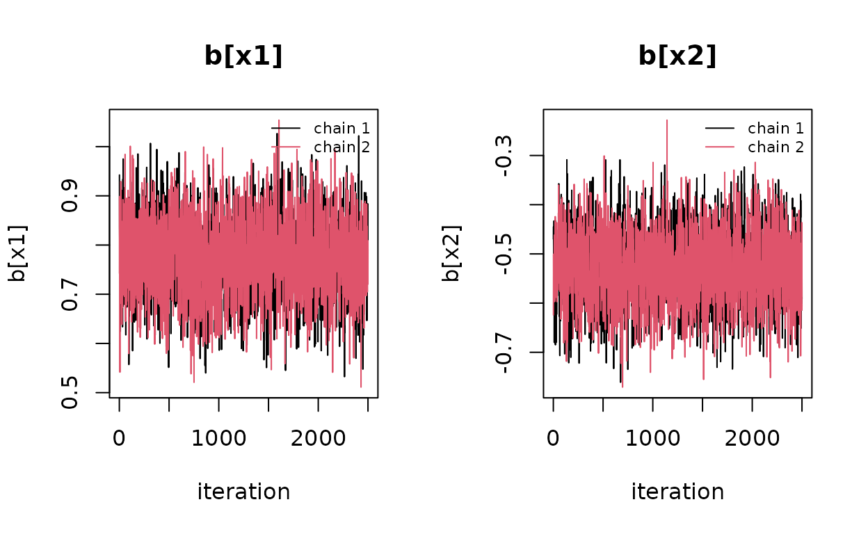

traceplot(fit, block = "delta")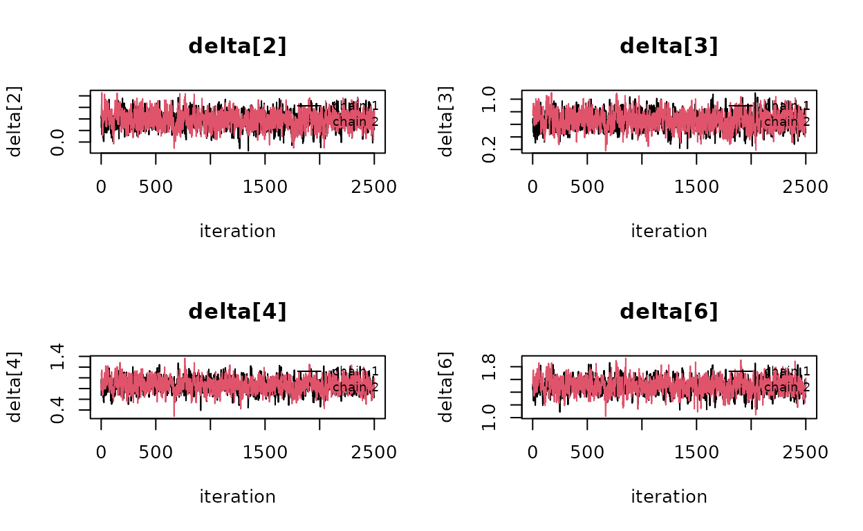

The same diagnostics are available programmatically, on any block, from the retained per-chain draws in fit$chains:

b_chains <- lapply(fit$chains, function(ch) ch$b)
rhat(b_chains, rank = TRUE)
#>     x1     x2 
#> 1.0016 0.9997
ess(b_chains)
#>    bulk tail
#> x1 2160 3456
#> x2 2093 3419
mcse(b_chains)
#>       x1       x2 
#> 0.001664 0.001550

Two chains keep this vignette build manageable and permit between-chain checks; for a serious empirical run, four or more chains are often a better default. choicer offsets the RNG seed across chains but currently gives them the same data-driven initialization, so this is not an overdispersed-start diagnostic. Report the number of people, tasks per person and alternatives; all prior scales; HMNL acceptance rates; rank-normalized R-hat; bulk and tail ESS; MCSE; trace plots; and posterior-predictive shares. Show prior sensitivity for W and sigma_d2. For entry, defend why the entrant’s residual quality is exchangeable with incumbents rather than treating the posterior predictive as a data-free ASC.

Did we recover the truth?

Because the data are simulated, we can line the posterior up against the generating parameters:

recovery_table(fit, sim)
#> <choicer_recovery> model=choicer_hmnl level=0.95
#>       parameter   group    true estimate     se    bias rel_bias_pct z_vs_true
#>          <char>  <char>   <num>    <num>  <num>   <num>        <num>     <num>
#>  1:          x1    beta  0.8000   0.7751 0.0764 -0.0249      -3.1151   -0.3261
#>  2:          x2    beta -0.6000  -0.5268 0.0711  0.0732     -12.1994    1.0295
#>  3:       W[x1]       w  0.5000   0.6243 0.1350  0.1243      24.8514    0.9206
#>  4:       W[x2]       w  0.5000   0.4567 0.1010 -0.0433      -8.6646   -0.4288
#>  5: (Intercept)   theta  0.5000   0.8588 0.3397  0.3588      71.7510    1.0561
#>  6:          z1   theta -0.4000  -0.3036 0.5380  0.0964     -24.1059    0.1792
#>  7:     sigma_d sigma_d  0.5000   0.5611 0.2609  0.0611      12.2134    0.2341
#>  8:           1   delta  0.4846   0.5427 0.1292  0.0581      11.9956    0.4500
#>  9:           2   delta  0.3525   0.3828 0.1350  0.0303       8.5995    0.2246
#> 10:           3   delta  0.6180   0.6616 0.1293  0.0435       7.0439    0.3366
#> 11:           4   delta  0.9914   0.8638 0.1271 -0.1276     -12.8663   -1.0037
#> 12:           5   delta  0.3393   0.5069 0.1302  0.1676      49.4109    1.2876
#> 13:           6   delta  1.4939   1.4971 0.1155  0.0032       0.2114    0.0273
#>     lower_ci upper_ci covers
#>        <num>    <num> <lgcl>
#>  1:   0.6253   0.9249   TRUE
#>  2:  -0.6662  -0.3874   TRUE
#>  3:   0.3597   0.8888   TRUE
#>  4:   0.2586   0.6547   TRUE
#>  5:   0.1930   1.5245   TRUE
#>  6:  -1.3580   0.7508   TRUE
#>  7:   0.0497   1.0724   TRUE
#>  8:   0.2895   0.7959   TRUE
#>  9:   0.1182   0.6473   TRUE
#> 10:   0.4081   0.9150   TRUE
#> 11:   0.6148   1.1129   TRUE
#> 12:   0.2517   0.7621   TRUE
#> 13:   1.2706   1.7235   TRUE

The population means b, the taste variances diag(W), and the realized $\delta_j$ ladder recover tightly. Note the pattern in the theta and sigma_d rows: with only $J = 6$ alternatives, the mean-function regression of $\delta$ on $z$ has six observations, so those posteriors are wide and lean on the prior — more alternatives is what sharpens them. The level of $\delta$ has its own identification story: it is pinned by the outside-option share, so with a small outside share the level posterior is diffuse while the cross-alternative contrasts stay tight.

Willingness to pay and predicted shares

Treating x2 as the price-like attribute, wtp() forms the per-draw ratio of population-mean utility coefficients and summarizes its posterior — a median and quantile interval rather than a delta-method approximation, so the ratio’s skewness is carried through honestly:

wtp(fit, price_var = "x2")
#>    attribute   wtp lower upper
#>       <char> <num> <num> <num>
#> 1:        x1 1.478 1.069  2.11

predict() integrates shares over both the taste distribution and the chain-1 posterior, returning posterior-predictive intervals (and the outside share):

set.seed(7)
predict(fit, n_draws = 200)
#>    alternative   share       sd   lower   upper
#>         <char>   <num>    <num>   <num>   <num>
#> 1:           1 0.12513 0.010228 0.10667 0.14489
#> 2:           2 0.10865 0.009731 0.09117 0.12711
#> 3:           3 0.13512 0.009445 0.11704 0.15344
#> 4:           4 0.16652 0.009865 0.14848 0.18804
#> 5:           5 0.11752 0.008488 0.10271 0.13338
#> 6:           6 0.28834 0.015315 0.25597 0.31456
#> 7:   (outside) 0.05872 0.009962 0.03849 0.07785

A posterior-predictive check compares observed choice shares with the model’s predictive distribution — a first-pass reality check on fit:

ppc_shares(fit, n_draws = 200)
#>    alternative observed predicted   lower   upper covered
#>         <char>    <num>     <num>   <num>   <num>  <lgcl>
#> 1:           1   0.1253   0.12501 0.10707 0.14527    TRUE
#> 2:           2   0.1073   0.10843 0.09232 0.12781    TRUE
#> 3:           3   0.1333   0.13487 0.11574 0.15454    TRUE
#> 4:           4   0.1680   0.16628 0.14821 0.18553    TRUE
#> 5:           5   0.1173   0.11757 0.09984 0.13274    TRUE
#> 6:           6   0.2907   0.28885 0.25556 0.31665    TRUE
#> 7:   (outside)   0.0580   0.05899 0.04182 0.08055    TRUE

Individual-level tastes are available too: fit$beta_i stores per-person posterior summaries (or full draws with keep_beta_i = "draws"), and predict(fit, level = "individual") conditions on them.

A policy counterfactual

Cut the price x2 of alternative 1 by 0.25 and re-predict — no refitting. Reusing the RNG seed makes the baseline and counterfactual share calculations use the same posterior and taste draws. This common-random-number pairing reduces Monte Carlo noise in the contrast; it does not make a finite-draw integral exact:

cf <- sim$data
cf$x2[cf$alt == 1] <- cf$x2[cf$alt == 1] - 0.25

set.seed(7)
base_shares <- predict(fit, n_draws = 200)
set.seed(7)
cf_shares <- predict(fit, newdata = cf, n_draws = 200)

data.frame(
  alternative    = base_shares$alternative,
  baseline       = round(base_shares$share, 3),
  counterfactual = round(cf_shares$share, 3)
)
#>   alternative baseline counterfactual
#> 1           1    0.125          0.138
#> 2           2    0.109          0.107
#> 3           3    0.135          0.133
#> 4           4    0.167          0.164
#> 5           5    0.118          0.116
#> 6           6    0.288          0.284
#> 7   (outside)    0.059          0.058

The welfare change is the posterior of the compensating variation — the logsum difference divided by the marginal utility of income, draw by draw:

set.seed(7)
cs <- consumer_surplus(fit, price_var = "x2", newdata = cf, n_draws = 200)
attr(cs, "cv")
#>   2.5%    50%  97.5% 
#> -68.17  41.75 208.81

The three numbers are the lower quantile, posterior median, and upper quantile of the sum of compensating variation over the prediction tasks. Supply weights = rep(1 / fit$nobs, fit$nobs) for an equally weighted mean, or a substantively justified task-weight vector for another aggregate. The function does not normalize user-supplied weights.

Unlike a delta-method standard error, this interval carries posterior uncertainty in the logsum and in the population-mean marginal utility of income $-\bar\gamma_{price}$ used as the denominator. This is a population-mean money metric, not the posterior distribution of person-specific compensating variation when marginal utilities of income differ across people. The taste distribution still enters the integrated logsum, and for a lognormal price coordinate it also enters $\bar\gamma_{price} = \exp(b + W_{kk}/2)$ . Report that aggregation choice explicitly in applications with price heterogeneity; an aggregate fixed-sign denominator does not by itself rule out individual price coefficients near or across zero. (logsum() and consumer_surplus() are available for the hierarchical logit only; the probit expected-maximum counterpart is on the roadmap.)

An entry counterfactual

The distinctive payoff of the BLP-style alternative level. A model with fixed alternative-specific constants is silent about an alternative it has never seen — it has no ASC for the entrant and no principled way to invent one. Here the entrant is a draw from the estimated population of alternatives: given its characteristics $z_{\text{new}}$ , each posterior draw assigns it $\delta_{\text{new}} \sim N(z_{\text{new}}'\theta_r,\; \sigma_{d,r}^2)$ .

Add the entrant’s rows to the data — same layout, a new alt label, its z1 value, choice = 0 — and predict:

entrant <- sim$data[sim$data$alt == 1, ]
entrant$alt <- 99L
entrant$z1 <- 0.4
entrant$choice <- 0L
entry_data <- rbind(sim$data, entrant)

set.seed(7)
predict(fit, newdata = entry_data, n_draws = 200)
#>    alternative   share      sd   lower   upper
#>         <char>   <num>   <num>   <num>   <num>
#> 1:           1 0.10003 0.01529 0.06639 0.12202
#> 2:           2 0.09367 0.01291 0.07470 0.11370
#> 3:           3 0.11648 0.01571 0.09082 0.13959
#> 4:           4 0.14408 0.01816 0.11948 0.16991
#> 5:           5 0.10138 0.01355 0.07956 0.12409
#> 6:           6 0.25022 0.03022 0.20973 0.29338
#> 7:          99 0.14399 0.09534 0.04630 0.29633
#> 8:   (outside) 0.05015 0.01025 0.03194 0.06843

The entrant takes share from every incumbent and from the outside good, and its credible interval is typically wider than the incumbents’ — appropriately so. The model knows the entrant’s observed characteristics but not its $\xi$ , so the prediction integrates over $\xi_{\text{new}} \sim N(0, \sigma_d^2)$ : the uncertainty about unobserved quality can be a dominant uncertainty about an entrant, and the posterior predictive exposes it rather than hiding it. The maintained assumption is exchangeability — the entrant’s unobserved quality is a draw from the same population as the incumbents’.

Price endogeneity

If a price-like covariate is correlated with the unobserved quality $\xi_j$ — the classic demand-estimation concern — the estimates are exogenous only conditional on $Z$ . The data preparations accept a control-function residual (cf_residual_col, Petrin and Train 2010): regress price on instruments outside the package, and pass the first-stage residual so it enters utility as an ordinary covariate. The package does not run the first stage, and posterior uncertainty does not propagate first-stage estimation error; joint Bayesian IV is on the roadmap.

The probit sibling

run_hmnprobit() estimates the same two-level structure with iid normal utility shocks instead of extreme-value ones. The sampler is fully conjugate (Albert-Chib data augmentation — no Metropolis step, no acceptance rates to tune), and because it works in un-differenced utility space, unbalanced choice sets pose no problem. The probit has a free scale, handled by parameter expansion: a non-identified $\sigma^2$ chain wanders by design, and every reported quantity is normalized per draw, so all summaries are on the identified scale. Do not diagnose convergence from the wandering, unidentified raw sigma2 chain alone; diagnose the normalized structural and predictive quantities that enter the economic conclusions.

simp <- simulate_hmnp_data(N = 250, T = 5, J = 6, seed = 42)

set.seed(99)
fitp <- run_hmnprobit(
  data               = simp$data,
  id_col             = "task",
  alt_col            = "alt",
  choice_col         = "choice",
  covariate_cols     = c("x1", "x2"),
  person_col         = "pid",
  alt_covariate_cols = "z1",
  chains             = 2,
  mcmc               = list(R = 30000, burn = 5000, thin = 10)
)
#> MCMC run time 0h:0m:14s
summary(fitp)
#> Hierarchical Bayesian Multinomial Probit (HMNP) model
#> 
#> Population coefficients b (posterior):
#> Parameter        Mean         SD       2.5%     Median      97.5%
#> x1           0.838019   0.064414   0.715976   0.836239   0.973327
#> x2          -0.668942   0.063487  -0.791690  -0.669136  -0.540771
#> 
#> Delta mean function theta (posterior):
#> Parameter          Mean         SD       2.5%     Median      97.5%
#> (Intercept)    0.736076   0.333940   0.030899   0.737186   1.402161
#> z1            -0.269438   0.563322  -1.373747  -0.278185   0.846182
#> 
#> Alternative-effect variance (posterior):
#> Parameter        Mean         SD       2.5%     Median      97.5%
#> sigma_d^2    0.417180   0.590158   0.089324   0.277676   1.547597
#> 
#> Raw shock variance (non-identified chain):
#> Parameter            Mean         SD       2.5%     Median      97.5%
#> sigma^2 (raw)    2.917235   1.327301   1.211681   2.701332   6.961030
#> 
#> Quality ladder (delta = mean utility vs the outside option; xi = delta - z'theta):
#>  alternative delta_mean delta_sd xi_mean  xi_sd
#>            1     0.2782   0.1086 -0.2343 0.3727
#>            2     0.3253   0.1085 -0.1753 0.3889
#>            3     0.5707   0.1050 -0.2807 0.5070
#>            4     0.9741   0.0991  0.4161 0.3117
#>            5     0.2759   0.1083 -0.3838 0.2646
#>            6     1.3851   0.0950  0.6594 0.3139
#> 
#> Convergence diagnostics (2 chains, 2500 draws each)
#> Block                R-hat  ESS_bulk  ESS_tail  MCSE(mean)
#> b[x1]                1.001      2683      4124      0.0012
#> b[x2]                1.000      2610      3530      0.0012
#> theta[(Intercept)]   1.000      3308      4453      0.0059
#> theta[z1]            1.000      5000      4362      0.0081
#> sigma_d^2            1.001      3848      4328      0.0100
#> sigma^2 (raw)^       1.075        22        34      0.2904
#> delta (J=6)         1.003*      583*     1497*         —
#> *worst: delta[3]
#> ^sigma^2 (raw) is the non-identified parameter-expansion scale (expected to not converge by design; excluded from the convergence-failure check).
#> Acceptance: conjugate — no acceptance step
#> 
#> Respondents: 250  Choice situations: 1250  Alternatives: 6 
#> Draws kept: 2500  Chains: 2 
#> MCMC run time 0h:0m:14s

The identified probit coefficients live on a different scale from the logit’s. A common variance-matching rule notes that the EV1 shock has standard deviation $\pi/\sqrt{6} \approx 1.28$ against the probit’s 1, and therefore multiplies probit coefficients by $\pi/\sqrt{6}$ for a rough comparison. This is not an exact transformation: normal and Type-I extreme-value shocks have different shapes, and coefficients also need matched utility specifications and data:

rbind(
  probit         = coef(fitp),
  "logit scale"  = coef(fitp) * pi / sqrt(6)
)
#>                x1      x2
#> probit      0.838 -0.6689
#> logit scale 1.075 -0.8580

The choicer_hb post-estimation suite — predict() (probabilities by a deterministic fixed-node one-dimensional Gauss-Hermite approximation), wtp(), elasticities(), diversion_ratios(), ppc_shares(), recovery_table() — is available through the same interfaces on the probit fit. The exceptions are logsum() and consumer_surplus(), which are logit-only as noted above.

References

Berry, S., Levinsohn, J. and Pakes, A. (1995). Automobile prices in market equilibrium. Econometrica, 63(4), 841-890.

Petrin, A. and Train, K. (2010). A control function approach to endogeneity in consumer choice models. Journal of Marketing Research, 47(1), 3-13.

Rossi, P. E., Allenby, G. M. and McCulloch, R. (2005). Bayesian Statistics and Marketing. Wiley.

Train, K. E. (2009). Discrete Choice Methods with Simulation (2nd ed.). Cambridge University Press.

Vehtari, A., Gelman, A., Simpson, D., Carpenter, B. and Bürkner, P.-C. (2021). Rank-normalization, folding, and localization: An improved R-hat for assessing convergence of MCMC. Bayesian Analysis, 16(2), 667-718.