Discrete choice from data to policy, in a dozen lines • choicer

choicer estimates discrete-choice models for applied economics. The likelihoods, analytical gradients and Hessians are written in C++ with OpenMP parallelization, so estimation is fast and scales to specifications with hundreds of alternative-specific constants. Just as important, one consistent post-estimation interface takes you from a fitted model to the quantities you actually report: fitted shares (population shares when the sampling design supports that interpretation), elasticities, diversion ratios, willingness-to-pay with standard errors, and the welfare effects of a policy counterfactual.

This vignette runs the whole workflow on a real data set in a few lines.

library(choicer)
set_num_threads(2) # set for CRAN compilation; raise this on your own machine

The data

mode_choice is the classic Greene & Hensher intercity travel-mode data: 210 travellers, each choosing among air, train, bus and car. It ships with the package in choicer’s long layout — one row per traveller and alternative.

data(mode_choice)
head(mode_choice, 4)
#>   id  mode choice wait travel vcost gcost income size
#> 1  1   air      0   69    100    59    70     35    1
#> 2  1 train      0   34    372    31    71     35    1
#> 3  1   bus      0   35    417    25    70     35    1
#> 4  1   car      1    0    180    10    30     35    1

wait (terminal waiting time) and travel (in-vehicle time) are in minutes; vcost is the travel cost. These vary across modes within a traveller, which is exactly what a choice model needs.

Fit a multinomial logit

Point at the identifier, alternative and choice columns, list the covariates, and fit. Alternative-specific constants are included by default.

fit <- run_mnlogit(
  data           = mode_choice,
  id_col         = "id",
  alt_col        = "mode",
  choice_col     = "choice",
  covariate_cols = c("wait", "travel", "vcost")
)
#> Optimization run time 0h:0m:0.01s
summary(fit)
#> Multinomial Logit (MNL) model
#> 
#> Parameter    Estimate  Std.Error  z-value  Pr(>|z|)  
#> wait        -0.096887   0.010342  -9.3683  0.00e+00  ***
#> travel      -0.003995   0.000849  -4.7043  2.55e-06  ***
#> vcost       -0.013912   0.006651  -2.0916  3.65e-02  *
#> ASC_train   -0.786669   0.602607  -1.3054  1.92e-01  
#> ASC_bus     -1.433640   0.680713  -2.1061  3.52e-02  *
#> ASC_car     -4.739865   0.867532  -5.4636  4.67e-08  ***
#> ---
#> Signif. codes:  '***' 0.001 '**' 0.01 '*' 0.05
#> 
#> Std. Errors: Analytical Hessian 
#> Log-likelihood: -192.889 
#> AIC: 397.777  | BIC: 417.86 
#> McFadden R2: 0.337 (adj: 0.317) | Hit rate: 0.738 
#> N: 210  | Parameters: 6 
#> Optimization time: 0.01 s
#> Convergence: 3 ( NLOPT_FTOL_REACHED: Optimization stopped because ftol_rel or ftol_abs (above) was reached. )

Estimation takes a fraction of a second. Travellers dislike waiting time, in-vehicle time and cost — all three coefficients are negative — and the summary() footer reports McFadden’s R² and the in-sample hit rate alongside the usual fit statistics.

Predicted shares

shares <- drop(predict(fit, type = "shares"))
names(shares) <- as.character(fit$alt_mapping[[2]])
round(shares, 3)
#>   air train   bus   car 
#> 0.276 0.300 0.143 0.281

barplot(shares, col = "steelblue", ylab = "Predicted share",
        main = "Predicted mode shares")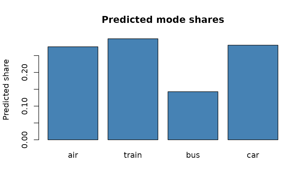

One thing this classic data set teaches well: the survey was choice-based — it deliberately over-sampled the minority modes and under-sampled car (see ?mode_choice) — so the shares above reproduce the sampling design, not population mode shares. The damage is contained in a useful way: in a logit with a full set of alternative-specific constants, choice-based sampling leaves the slope coefficients consistent (Manski and Lerman 1977), so the willingness-to-pay ratios below are unaffected, while the constants — and the share, elasticity and surplus levels computed from fitted probabilities — inherit the design. We proceed unweighted because the workflow, not the level estimates, is the point here; the correction is a weighting, not a different model, and it is the subject of the choice-based sampling vignette.

Elasticities and diversion

How does demand respond to cost, and where does it go? The same fitted object fit answers both, with no extra bookkeeping.

To recover elasticities with respect to the vcost variable, simply run

elasticities(fit, elast_var = "vcost")
#>           air   train      bus      car
#> air   -0.8309  0.1679  0.06729  0.06912
#> train  0.3551 -0.5463  0.06729  0.06912
#> bus    0.3551  0.1679 -0.39815  0.06912
#> car    0.3551  0.1679  0.06729 -0.22296

The own-cost elasticities sit on the diagonal; off-diagonal entries are the cross-elasticities. For example, the own-elasticity of train mode is -0.546, and the cross-elasticity from train to bus is ~0.17.

The corresponding diversion matrix answers a slightly different question: among the travellers who leave one mode after a marginal cost increase, where do they go?

diversion_ratios(fit)
#>          air  train    bus    car
#> air   0.0000 0.2776 0.2513 0.3860
#> train 0.3080 0.0000 0.3556 0.4144
#> bus   0.1719 0.2192 0.0000 0.1996
#> car   0.5201 0.5032 0.3931 0.0000

Columns indicate the origin and rows the destination. In this fit, a marginal increase in train’s cost diverts the displaced travellers roughly 28% to air, 22% to bus and 50% to car.

The MNL makes this calculation especially transparent. Conditional on the included covariates, diversion is governed by fitted choice probabilities rather than by an unobserved notion of closeness among alternatives. That is a useful baseline, and also a restriction. If the empirical object turns on grouped substitution, unobserved taste heterogeneity, or counterfactuals in which the composition of the choice set changes, the nested logit, mixed logit, and multinomial probit move that substitution structure in different directions. The comparison is summarized in Choosing among choice models below.

Willingness to pay

With vcost playing the role of price, wtp() returns the marginal value of each attribute in money units, with delta-method standard errors.

wtp(fit, price_var = "vcost")
#> Willingness to pay (WTP), price variable: 'vcost' (95% CI)
#>        Estimate Std_Error z_value CI_lower  CI_upper
#> wait    -6.9645    3.4085  -2.043 -13.6450 -0.283902
#> travel  -0.2871    0.1436  -2.000  -0.5685 -0.005757

These are the travellers’ implied value of time: how much they would pay to shave a minute of in-vehicle or terminal time.

A policy counterfactual

Suppose a subsidy cuts the cost of train travel by 25%. Perturb the data and predict — no refitting required.

mc_cf <- mode_choice
mc_cf$vcost[mc_cf$mode == "train"] <- mc_cf$vcost[mc_cf$mode == "train"] * 0.75

shares_cf <- drop(predict(fit, type = "shares", newdata = mc_cf))
names(shares_cf) <- names(shares)

rbind(baseline = shares, counterfactual = shares_cf) |> round(3)
#>                  air train   bus   car
#> baseline       0.276 0.300 0.143 0.281
#> counterfactual 0.269 0.324 0.138 0.270

Train’s share rises, drawing travellers away from the other modes. We can put a money value on the change in welfare with the expected consumer surplus:

cs0 <- consumer_surplus(fit, price_var = "vcost")
cs1 <- consumer_surplus(fit, price_var = "vcost", newdata = mc_cf)

cs1$mean_cs - cs0$mean_cs # change in mean consumer surplus
#> [1] 3.2

The cheaper train fare raises expected consumer surplus, as it should. The number is a model-based demand calculation, not a causal estimate by itself: it inherits the maintained utility specification — including linearity in cost, which fixes the marginal utility of income and rules out income effects (Train 2009, Ch. 3) — the price coefficient, and the assumption that the counterfactual changes only the variables you changed in newdata.

One interface, every model

Everything above — predict(), elasticities(), diversion_ratios(), wtp(), consumer_surplus(), plus blp() for share inversion — is also available on mixed logit (run_mxlogit()) and nested logit (run_nestlogit()) fits, with model-specific arguments where the economic object differs (notably the perturbation coordinate for MXL diversion). choicer also offers Bayesian samplers: a multinomial probit (run_mnprobit()) and hierarchical logit and probit models (run_hmnlogit(), run_hmnprobit()) with panel random coefficients and BLP-style alternative effects. Learn each model in its own vignette:

Multinomial logit — the workhorse, and a parameter-recovery check
Mixed logit — random coefficients and preference heterogeneity
Nested logit — grouped substitution through nests
Bayesian multinomial probit — correlated utility shocks via MCMC
Hierarchical Bayes — panel tastes, partially-pooled product effects, and entry counterfactuals

Two further vignettes cover inference and sampling design:

Which standard errors, and when — Hessian, BHHH, robust and cluster-robust variances, recomputable post hoc via vcov()
Choice-based sampling and WESML weights — estimation when the sample was drawn by outcome

Choosing among choice models

The useful starting point is not the name of the model. It is the object you intend to report. Own-price elasticities, diversion ratios, WTP, logsum welfare, entry effects and merger simulations put different demands on a model’s substitution structure and taste heterogeneity. A model that reproduces observed shares can still give poor answers to a counterfactual if the relevant substitution margin is supplied mainly by functional form.

choicer v0.2.0 supplies diversion and demand-side counterfactual ingredients, but it does not implement a merger-equilibrium simulator; merger analysis also requires a supply model, conduct assumptions, and a price-equilibrium solve.

For that reason, the model choice question is:

What variation identifies the substitution pattern needed for the object I want to report?

IIA is one implication of the MNL at the individual level: conditional on covariates, the odds between two alternatives do not depend on the rest of the choice set. That fact is worth knowing, but it should not organize the empirical discussion. The important question is which restrictions generate substitution beyond observed covariates, and whether the data contain variation that can discipline the corresponding parameters.

Model	What supplies substitution structure?	What has to be defended?
Multinomial logit	Included covariates and observed heterogeneity across choice situations.	The maintained utility index and the absence of unobserved closeness among alternatives. Individual-level diversion is proportional to fitted choice probabilities.
Nested logit	Shared unobservables within pre-specified nests, summarized by one dissimilarity parameter per nest.	The nesting tree and the random-utility interpretation of the estimated dissimilarity parameters. Correlation exists only where the tree permits it.
Mixed logit	A mixing distribution $f(\beta)$ for tastes, possibly with correlated random coefficients.	The distributional family, its tails, simulation accuracy, and the variation that identifies heterogeneity. choicer’s `run_mxlogit()` is cross-sectional and does not exploit persistence across repeated choices; use HMNL when one taste draw should persist within person.
Multinomial probit	A covariance matrix for utility-difference shocks.	Scale normalization, a rapidly growing covariance parameterization, and MCMC diagnostics. Alternative-varying covariates and defensible exclusions across utility equations help separate systematic utility from covariance (Keane 1992). choicer does not yet provide MNP prediction or a rule for transporting covariance to counterfactual choice sets.
Hierarchical MNL	Persistent taste heterogeneity $\beta_i \sim N(b, W)$ plus partially-pooled alternative effects $\delta_j = z_j'\theta + \xi_j$ , with iid EV1 choice shocks.	The priors, MCMC convergence, and—for entry counterfactuals—the exchangeability of entrant residual quality with incumbents. Repeated choices plus useful within-person variation are what discipline the taste distribution.
Hierarchical MNP	The same panel tastes and alternative hierarchy, with iid normal utility-level shocks and a stochastic outside option.	Per-draw scale normalization, normal-only random coefficients, and the iid shock restriction. Unlike `run_mnprobit()`, HMNP does not estimate an unrestricted utility-difference covariance; expected-maximum welfare is not implemented.

In practice, a mature research design can be organized around seven questions. They are deliberately about the empirical object rather than a preferred estimator.

What is the estimand and decision environment? State whether the target is a utility slope, WTP ratio or distribution, substitution pattern, population share, welfare contrast, or entry effect. Define the baseline and counterfactual menus, who faces them, and the horizon over which adjustment is allowed. An own-price elasticity on the observed menu may need less structure than diversion after exit, entry by a new product, or welfare under a menu the data have never observed.
What population and sampling design connect the data to that estimand? Define the choice situation, availability set, outside option, sampling unit, and aggregation weights. Distinguish sample shares from population or market shares. For a choice-based sample, document the source, population, date, and uncertainty of the external shares $Q$ ; WESML transports the likelihood to that population but does not make uncertain benchmark totals known.
Which variation identifies systematic utility and which assumptions make it exogenous? Map each coefficient to within-choice-set, across-market, experimental, or panel variation. Ask whether prices, waiting times, product availability, or hospital quality respond to latent demand. Neither a richer covariance model nor robust standard errors repair an endogenous utility shifter; instruments, a defensible control function, or another research design must supply that argument.
What supplies substitution beyond observed utility? Make explicit what is normalized, excluded, pooled, or supplied by iid shocks, a nesting tree, the tails of $f(\beta)$ , an unrestricted probit covariance, or the hierarchical alternative distribution. A model can reproduce observed shares while its policy substitution comes mainly from one of these maintained restrictions.
Does the data variation earn the model’s flexibility? A thin cross-section with one choice per person and a nearly fixed menu rarely disciplines a rich taste distribution. A motivated nest may be more credible than weakly identified random coefficients; repeated tasks with useful attribute variation can earn persistent panel tastes; many alternatives with informative $Z$ can earn an alternative-level hierarchy. Use the simplest model that carries the margin required by Question 1, not the model with the longest parameter vector.
How will uncertainty and computation be audited? Match the variance to the design: inverse Hessian under the maintained likelihood, a robust sandwich for misspecification or WESML, and clustering for dependent sampling units. For Bayesian fits, report priors, chains, rank-normalized R-hat, bulk and tail ESS, MCSE, traces, and posterior-predictive checks. For simulated likelihood, report starts, scaling, draw construction and stability as $S$ increases. Numerical convergence is necessary evidence, not identification.
Which diagnostics and sensitivity exercises could change the conclusion? Report fit, but stress-test the economic object: elasticities, diversion, WTP, welfare, and entry predictions across plausible utility specifications, nesting trees, mixing distributions, priors, population shares, simulation draws, and counterfactual support. If the conclusion moves with a tree, a tail, $Q$ , or an entrant-exchangeability assumption, that movement is part of the empirical result rather than a nuisance to suppress.

Question 3 deserves special emphasis: is the price coefficient itself credibly identified? If prices respond to unobserved demand — the standard concern whenever unobserved quality feeds both purchases and pricing — every row above is contaminated equally, and no amount of substitution structure repairs it. Model choice and price endogeneity are orthogonal problems. choicer’s tools for the latter follow the control-function tradition (Petrin and Train 2010): run the first stage of price on instruments outside the package and include the residual as an ordinary covariate (the hierarchical Bayes data preparations have a dedicated cf_residual_col argument). For market-level data, note that blp() is the inversion step of Berry (1994) — it recovers the mean utilities that rationalize observed shares, which can then be regressed, with instruments, on characteristics and price.

Each model’s own vignette develops these tradeoffs in detail: MNL, nested logit, mixed logit, hierarchical Bayes.

How choicer compares

Several excellent R packages estimate discrete-choice models — among them mlogit, logitr, gmnl, apollo and mixl. choicer’s focus is a fast C++ core with analytical gradients and Hessians, and a single, consistent post-estimation toolkit aimed at the demand and welfare quantities applied economists report.

References

Berry, S. (1994). Estimating discrete-choice models of product differentiation. RAND Journal of Economics, 25(2), 242-262.

Keane, M. P. (1992). A note on identification in the multinomial probit model. Journal of Business & Economic Statistics, 10(2), 193-200.

Manski, C. F. and Lerman, S. R. (1977). The estimation of choice probabilities from choice based samples. Econometrica, 45(8), 1977-1988.

Petrin, A. and Train, K. (2010). A control function approach to endogeneity in consumer choice models. Journal of Marketing Research, 47(1), 3-13.

Train, K. E. (2009). Discrete Choice Methods with Simulation (2nd ed.). Cambridge University Press.